

11.0 Mathematical Modeling of thermoelectric Cooling Modules
11.1 INTRODUCTION: The operation of thermoelectric cooling devices may be described mathematically and device performance can readily be modeled on a personal computer. Since the semiconductor material used in module fabrication has several temperature-dependent properties, temperature effects on module operation must be considered if a realistic model is to be developed. We have not attempted to provide a highly detailed description of computer modeling techniques, but rather to present the basic algebraic expressions needed to simulate thermoelectric module performance.
Ferrotec America has performed a comprehensive analysis of many thermoelectric cooling modules over a wide temperature range. This study has resulted in the development of mathematical models that may be used to reliably predict module performance under typical operating conditions. Data presented herein is based on module operation in a normal air atmosphere with thermally conductive grease (heat sink compound) used at both hot and cold module interfaces. These conditions are applicable to the majority of thermoelectric cooling applications. It should be noted that for modules having metabolized external surfaces, slight performance improvement may be observed if the modules are mounted with solder as opposed to thermal grease. In addition, when modules are operated in a vacuum, a small to moderate performance increase may be seen, especially in the case of multi-stage devices.
11.2 TEMPERATURE-DEPENDENT MATERIAL PROPERTIES: There are a number of parameters associated with thermoelectric materials and modules that normally would have to be considered in a mathematical model. However, since actual module test data was used to derive several important coefficients, certain factors may be neglected thereby simplifying the modeling process. Elements that must be incorporated into the model include the module's effective Seebeck coefficient (SM), Electrical Resistance (RM), and Thermal Conductance (KM).
The values of SM, RM, and KM can be expressed mathematically by polynomial equations. The specified equation coefficients, applicable over a range of -100°C to +150°C, were derived from an industry-standard 71-couple, 6-ampere module. Other module configurations easily can be modeled by applying a simple correction factor as described in paragraph 11.2.4. Note that when using the various equations, temperature values must be stated in degrees Kelvin.
An alternative method for estimating temperature-dependent module properties, which may be useful under certain circumstances, involves the use of tabulated module data. Values representing average SM, RM, and KM characteristics for selected modules over a wide temperature range will be found in Appendix A at the end of this manual. Although somewhat less accurate than using calculated values, this method provides a relatively simple approach to predicting module performance.
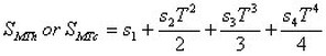
11.2.1 SEEBECK COEFFICIENT: When a temperature differential is maintained across a thermoelectric device, a voltage can be detected at the input terminals. The magnitude of the resultant voltage, called the Seebeck emf, is proportional to the magnitude of the temperature difference. The Seebeck coefficient, as a function of temperature, can be expressed as a third order polynomial:
![]()
Where:
SM is the Seebeck coefficient of the module in volts/°K
T is the average module temperature in °K
Coefficients for a 71-cpl, 6-amp module
s1 = 1.33450 x 10E-2
s2 = -5.37574 x 10E-5
s3 = 7.42731 x 10E-7
s4 = -1.27141 x 10E-9
The above polynomial expression represent the Seebeck coefficient when the temperature difference across the module is zero (DT = Th - Tc = 0). When DT>0, the Seebeck coefficient must be evaluated at both temperatures Th and Tc using the expressions:
![]()
Where:
SMTh is the module's Seebeck coefficient at the hot side temperature T
SMTc is the module's Seebeck coefficient at the cold side temperature Tc
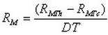
11.2.2 MODULE RESISTANCE: The electrical resistance of a thermoelectric module, as a function of temperature, can be expressed as third order polynomials for the two conditions (a) and (b):
(a) when DT = 0:
![]()
(b) when DT > 0:
![]()
Where:
RM is the module's resistance in ohms
RMTh is the module's resistance at the hot side temperature Th
RMTc is the module's resistance at the cold side temperature Tc
T is the average module temperature in °K
Coefficients for a 71-cpl, 6-amp module
r1 = 2.08317
r2 = -1.98763 x 10⁻²
r3 = 8.53832 x 10⁻⁵
r4 = -9.03143 x 10⁻⁸
11.2.3 MODULE THERMAL CONDUCTANCE: The thermal conductance of a thermoelectric module, as a function of temperature, can be expressed as third order polynomials for the two conditions (a) and (b):
(a) when DT = 0:
![]()
(b) when DT > 0:
![]()
![]()
Where:
K is the module's thermal conductance in watts/°K
KMTh is the thermal conductance at the hot side temperature Th
KMTc is the thermal conductance at the cold side temperature Tc
T is the average module temperature in °K
coefficients for a 71-cpl, 6-amp module
k1 = 4.76218 x 10⁻¹
k2 = -3.89821 x 10⁻⁶
k3 = -8.64864 x 10⁻⁶
k4 = 2.20869 x 10⁻⁸
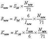
11.2.4 PARAMETER CONVERSIONS FOR OTHER MODULE CONFIGURATIONS: The SM, RM, and KM parameters shown are calculated for a 71-couple, 6-ampere thermoelectric module. If a new or different module configuration is to be modeled, it is necessary to apply a conversion factor to each of these parameters, as follows:
Where:
Snew is the Seebeck coefficient for the new module
Rnew is the electrical resistance of the new module
Knew is the thermal conductance of the new module
Nnew is the number of couples in the new module
Inew is the optimum or maximum current of the new module
11.3 CALCULATION OF THERMOELECTRIC MODULE PERFORMANCE: There are five variable parameters applicable to a thermoelectric module that affect its operation.
These parameters include:
In order to calculate module performance it is necessary to set at least three of these variables to specific values. Two common calculation schemes involve either (a) fixing the values of Th, I, and Qc or, (b) fixing the values of Th, I and Tc. For the computer-oriented individual, a relatively straightforward calculation routine can be developed to incrementally step through a series of fixed values to produce an output of module performance over a range of operating conditions.
11.4 SINGLE-STAGE MODULE CALCULATIONS: These equations mathematically describe the performance of a single-stage thermoelectric module as illustrated in Figure (11-l). When entering numerical data, do not forget that temperature values must be expressed in degrees Kelvin (°K). Calculations of the various parameters should be performed in the order shown.
Figure (11-1)
a) The temperature difference (DT) across the module in °K or °C is:
DT = Th - Tc
b) Heat pumped (Qc) by the module in watts is:
![]()
c) The input voltage (Vin) to the module in volts is:
![]()
d) The electrical input power (Pin) to the module in watts is:
Pin = Vin x I
e) The heat rejected by the module (Qh) in watts is:
Qh = Pin + Qc
f) The coefficient of performance (COP) as a refrigerator is:
COP = Qc / Pin
11.5 HEATING MODE OPERATION: Thermoelectric modules may be operated in the heating mode by reversing the polarity of the applied DC power. When used in this manner, the TE module functions as a "heat pump" and heating efficiencies in excess of 100 percent may be realized under certain conditions. A rapid increase in temperature occurs when heating a small-mass object, and care must be taken to avoid overheating either the module or object. In the heating mode, illustrated in Figure (11-2), the heat sink and object effectively are in opposite positions whereby the object is now at temperature (Th) and the heat sink is at temperature (Tc).

Figure (11-2) a) Heat flow to the object (Qh) is given by the expression:
![]()
b) The coefficient of performance as a heater (COPH) is:
COPH = Qh / Pin
11.5.1 Heating mode performance of a standard 71-Couple, 6-Ampere module is presented graphically in Figures (11-3) and (11-4). These graphs illustrate module performance at a heat sink temperature of 25°C.
Figure (11-3)
Heat Output at Various Hot-Side Object Temperatures
Figure (11-4)
Coefficient of Performance in the Heating Mode
11.6 OTHER THERMOELECTRIC DEVICE ATTRIBUTES: There are many other properties of thermoelectric devices that can be described mathematically. Several characteristics that might be of interest for specific situations follow. Remember that temperature values must be expressed in °K.
a) The maximum heat pumping capacity (Qmax) in watts of a thermoelectric module is given by the following expression. Note that DT =0 at the maximum Qc condition and, therefore, Tc = Th.
![]()
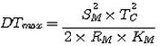
b) The maximum temperature differential (DTmax) in °K may be expressed as shown below. To obtain an accurate DTmax value, however, it will be necessary to perform an iterative series of calculations comparing Tc to DTmax at a fixed value of Th.
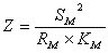
c) The Figure-of-Merit (Z) is a measure of the overall performance of a thermoelectric device or material. Z always is higher for raw thermoelectric semiconductor material than for an actual module functioning within a thermal system. Since an operating module is affected by interface, conductive, convective, and other losses, the effective Figure-of-Merit is less than that of the raw material.
The Figure-of-Merit may be expressed:
For Raw Material:

For a TE Module:
where:
a is the Seebeck coefficient of the material in v/°K
p is the electrical resistivity of the material in ohm-cm
k is the thermal conductivity of the material in w/cm-°K
d) The optimum current (Iopt) in amperes required to produce the maximum heat removal rate (Qmax) is:
For Raw Material:
![]()
For a TE Module:
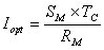
where:
a is the cross-sectional area of an individual thermoelectric element in centimeters.
l is the length (height) of an individual thermoelectric element in centimeters
R is the resistance of an individual thermoelectric element in ohms.
11.7 MODELING OF COMPLETE THERMOELECTRIC COOLING SYSTEMS: Information presented in the foregoing paragraphs describes the mathematical modeling of thermoelectric modules as opposed to complete thermal systems. By incorporating the module calculations into a more sophisticated system model, it is possible to accurately simulate the overall thermal performance. Two heat leak sources that must not be overlooked in a complete thermal model include (a) heat conduction between the cooled object and heat sink, and, (b) heat conduction through clamping screws, if any, that physically connect the heat sink and cooled object.
Heat conduction between the heat sink and object generally involves the transfer of heat through the air gap surrounding the module mounting area. The actual heat leak value can be calculated using the equation in paragraph 8.4.1 where area (A) is the "open" surface area not covered by the thermoelectric modules, distance (x) is the width of the air gap, and thermal conductivity (K) is the value for air.
Heat conduction through the clamping screws also can be calculated by means of the same equation. In this case, area (A) is the cross-sectional area of all mounting screws calculated from the screw's pitch diameter and (K) is the thermal conductivity of the screw material.